9 Tools To Manipulate Data In Excel

Table of Contents

Flash Fill And Remove Duplicates
Sharing Excel Files
Filtering Data
What Is Flash Fill?
Split Data Into Separate Cells
Naming Excel Sheets
Navigating Multiple Sheets
Navigating Large Microsoft Excel Spreadsheets
To Double Click Or Not To Double Click
Conclusions

Flash Fill And Remove Duplicates

If you deal with lots of data lists and find yourself doing a lot of cleaning and tiding up as well as having Microsoft Excel version 2013 or higher, then you will have this new feature called Flash Fill.

Prior to this version you will need to use the usual Text to Column feature found under the Data Tab. When you have data like an email address you may be needing to display only the surname. See “What Is Flash Fill In Excel” for examples.

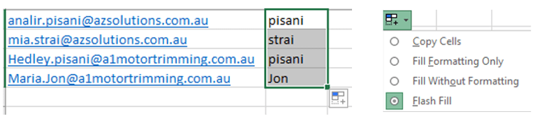
With Microsoft Excel’s Flash Fill you can start the ball rolling by typing in the next column, for example the surname “Pisani” then fill the contents of the cell down. Initially the data should repeat. From the AutoFill Smart Tag that appears select Flash Fill this will start to pick up the surname from each row.

Microsoft Excel now has a feature called Remove Duplicates found under the Data Tab. Just take note the result of the duplicates does not get re located onto a separate sheet so once you press that button – Remove Duplicates, that’s it, you are left with the clean data.

In the past the alternative was to sort data then create an If Statement to test the first cell with the one below and return Yes or No, then filter all the yes’s and delete.

Sharing Excel Files

Sharing Excel Files using One Drive is very easy. One Drive is a Microsoft Office product that’s why it plays well with other Microsoft Office products like Excel.

One person can be in the file making a change and at the very same time another can be seeing the changes take place right before their eyes.

1. Open the Excel File
2. If you have version 2013 or 2016 you will have a share icon on the top right-hand corner
3. Click the Share button
4. Select Save to Cloud
5. From the left-hand side Select OneDrive
6. From the right navigate through your OneDrive folders
7. Double Click the OneDrive folder to store it in
8. Make sure you name your file then Press Save

Filtering Data

We can use Microsoft Excel when dealing with long lists. There are several techniques you can use to achieve this. One is to Go to the Data Tab and Select the Filter button the Second option is to activate from the Home tab and Select Filter.

Whilst the Filter tool is useful and will show you only the data that you are interested in. It also has the sort feature built into it under the Drop-down arrows.

Important to note is if you have blank rows and select a cell at the top, your filter will only capture data up until there was a blank row. What you should do first is select the first cell of your data, Press Ctrl Shift End then press the Data Tab and Select Filter.

The feature I love the most in the Filters is the Search Bar. Press the down arrow of any heading you will then see the Search Bar. If you have dates you can group quickly and easily by quarter, this quarter, last quarter. I find this so handing when importing my bank statements into Excel and then doing my book work.

Filter By and Sort By colour are both great tools to gather information for example everything yellow needs a post code, everything green is completed.

What Is Flash Fill?

An alternative to using Text to Column to extract the part that you need from a mix of data is the Flash Fill feature in Excel.

For example, if you have: analir.pisani@azsolutions.com.au you might want to extract each person’s surname.
Alternatively use Text to Column found under Data Tab.

1. Type Pisani then fill down
2. Click on the AutoFill Options Smart Tag
3. Select Flash Fill only available since version 2013 forward

Split Data Into Separate Cells

When you need to split the data in Microsoft Excel from one column into several – use Text to Column. You can split the data each time there is a: space, comma, @, Tab and more. This feature has been available for many versions of Microsoft Excel.

Split a comments field which has Alt Enter text. Text in the same cell but on a new line. To Separate these use the Delimited option as the Other type:

Ctrl J. You will not see the letter J in the box but the action will work. Trust in the Force. 😉

What is new since Microsoft Excel Version 2013 is Flash Fill. Most of the time when people are using the Text to Column feature, they are not aware that they can skip columns. So, what they do is bring everything in and then start deleting columns when they could have done it in one place. Same goes for formatting the feature to format as date is in the Text to Column dialog box.

Here are the steps to separate data from on column into several columns.

Using Text To Column

1. 1. Select the column to split
   2. Ensure there is no data to the right
   3. Go to the Data Tab
   4. Select Text to Column
   5. If the data is separated by spaces, tabs, commas us the delimited options
   6. If the data has no notable separator use fixed
   7. If there is a column you do not wish to display
   8. Select “Do not import column(skip)”

Naming Excel Sheets

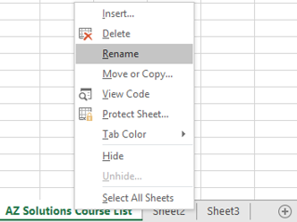
There are two techniques you can use when wanting to name your sheets in Microsoft Excel. You can Double Click on the name of the sheet, type the name and press Enter. You can also Right Mouse Click on the name of sheet and select from the list, Rename.

When working in Microsoft Excel you have a Workbook Name which means the name of the file. In just one sheet you have 16,000 columns and over 1 million rows.

English pages and pages worth of data in just 1 sheet. To navigate efficiently through all these sheets, you might like to Right Mouse Click on the arrows on the bottom left-hand corner. This will display a list of all the names of the sheets in your Microsoft Excel Workbook.

No, they do not appear in alphabetical order.

They appear in the order that you need to work with them. You can also Right Mouse Click on the Name of the sheet to change its tab colour, this can make it easier to find.

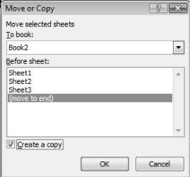
To make a copy of a sheet you can Right Mouse Click and select Move or Copy but it’s much easier if you hold the CTRL key as you drag. You should see a plus sign, this means it’s performing a copy.

YouTube Working with Sheets

This video will walk you through how to create a new sheet, rename it, copy a sheet and group sheets. The best thing about grouping sheets is that once they are grouped whatever you do in one cell will display in each of the other sheets. Imagine the formula or function was incorrect for each department sheet in cell A50. Group your sheets, make the change ungroup the sheets, that’s it they are all done all 20 different department sheets you had.

Navigating Multiple Sheets

If you find yourself working between multiple sheets you may find it frustrating to get quickly from one to the other. Pressing the navigation arrows on the bottom left will take for ever.

You could use shortcut keys Ctrl Page Up, Ctrl Page Down but this isn’t any faster.

Try the ultimate “Right Mouse Click” on the bottom left navigation arrows.

You will be presented with a list of all your sheets simply select one item in the list initially then press the first letter of the sheet name you would like to get to. If it didn’t get to the one you wanted, continue pressing the same letter. It will cycle through everything that starts with that letter.

Navigating Large Excel Spreadsheets Efficiently

Excel Spread sheets can be a pain to get around when you have lots of sheets to bounce around between and data that spans over many columns and rows.

Ctrl Home and Ctrl End should be the first keystrokes you ever learn because these can be used in not only Microsoft Excel Products but also in Word and PowerPoint. Ctrl Home will get you to the top and Ctrl End will get you to the very last page if in Word or the last column or row that has data in it for Excel.

I don’t know about you, but I found it stressful when I started a new job and I had to navigate someone else’s Excel spread sheets. I kept getting lost bouncing between the sheets that I needed to play with.

Sometimes I have coloured the sheets that are relevant to me. That worked.

Best Solution: Using the navigation arrows at the bottom left hand side. Right Mouse Click on them. This will produce a list of all the sheets in your workbook. Select the one you want, and press enter. It now takes you directly to that sheet. Stress solved. Ok one stress solved.

Selecting chunks of data is another drama. Click and drag for 100 years. Then I go past what I needed and fine it frustrating to go back. I’ve lost the plot by then.

If you have a block of data up to the point where there is a blank row or column. Ensure you have clicked inside that data set. This part of the step is crucial. Two keys and you’re done. CTRL A. Then you can continue to do whatever you like with this selected set. Copy and paste it, do some formatting or delete it.

Excel Shortcut Keys You Really Need To Know

If you change your mind and need to select the whole sheet you already pressed CTRL A when you were inside the data set press CTRL A, a second time and this will extend the selection to the entire Excel Sheet.

Saving your Excel spreadsheets as you go along is crucial. You can press the Save icon from the Quick Access Toolbar or you can save yourself a lot of time and press Ctrl S. Sometimes what you are after is not quite save but Save As, in that instance press F12.

We tend to work with multiple opened workbooks at a time and get slack at cleaning up after ourselves as we go by closing the files we don’t need. This is often why our machines struggle; they don’t have enough ram power to keep everything open. When you are ready to clear your Excel desk of opened files Hold the Shift key as you press the close cross at the top right-hand corner. This will close all your currently opened Excel Workbooks. Ctrl W will close only the current Excel Workbook.

If you are the kind of person that saves everything onto the Desktop, then getting to the Desktop when you are in an application can be done in several different ways. First you can close every Application window you have open until you can see the desktop. To the far right of your Windows Task Bar, where you can hardly see a command button area, you can click it and you will get to the Desktop. Are you ready for the ultimate keystroke Windows D?

Sure, it’s not hard to insert and Excel Worksheet you just press the plus sign all the way at the very end. When you press the plus sign, it inserts and Excel sheet to the right of the selected sheet. If you press Shift F11 you get the sheet inserted to the left of the selected sheet.

Ctrl Home you may already know will get you to cell A1.

When you work with extremely large Excel Worksheets that go into the double and the triple column letters. You will be looking for the quickest way you can find to get you to the very last column or row that has some data in it. Try, Ctrl End and Ctrl Shift End to Select and jump to the very end.

If creating graphs is something you need to do quite often. Well I’ve got one key for you. All you need is data with header labels and labels to the left then figures in each row. Ensure your cursor is in the data you don’t even have to have all the cells selected and then press F11. This will create a column graph for you.

Is data entry more your thing, are you typing the current date all the time perhaps for your time sheets. Don’t know about you but when I need to type todays date, I go looking at the bottom right-hand side of the Tabs bar. With this keystroke you will never look at the task bar or go for your phone to find the date. Press Ctrl ; and for the time press Ctrl Shift :

Pasting data is Ctrl V not Ctrl P. Ctrl P is for printing.

Insert Multiple Rows At A Time

Need to insert 5 to 10 rows above a certain point in your spreadsheet. I have seen people Right Click on ONE row and insert a row only to then repeat the process 5 times. There must be an easier way right. Yep there is.

Select 5 to 10 rows first then Right Mouse Click and select insert rows. Woo-Hoo done. Hope your feeling excited about how much time you can save. Want more.

This video will give you great insights into how to Navigate and Select using Microsoft Excel spread sheets.

To Double Click Or Not To Double Click

I often get asked by customers starting out using computers for the first time. Do I Click once or twice?

Good question.

One click is to select an item or a command.

Double click is generally used when you want to open something.

Let us look at the example of Excel.

When you are in a cell and you want to edit the contents of that cell, the standard is that you can double click. Then proceed to make what ever changes you would like followed by pressing Enter.

Recently I had installed an adding for Excel called Power-user. This is the only change that I could think of that I had made to Excel. So, I had thought this had caused the problem or setting to be turned off. Since then I went to double click in a cell as usual to make an edit. It wouldn’t put me in edit mode. This happened when I was in the middle of a class demonstrating.

I did all the usual steps that should fix the problem. I saved and exited the file. Re opened the file. Still the same problem.

A student of mine then said I turn of a feature in Excel, so it does not edit the cell but instead takes me to the link or cell it references to.

File/ Options/ Advanced. Untick “Allow editing directly in cells”

Sure, enough I went to File/ Options/ Advanced and it was unticked so odd. I certainly didn’t untick this feature.

It so happens that this is something that I actually have had students ask me.

Scenario: I have a cell with a link to data in a different sheet. For example =Finance!G20. I want to click on the cell that refers to another location and I also want to be able to come back.

With this feature turned on you can Double click on the cell to jump to for example Finance cell G20. Now to come back you will need to press F5 or the Go to command and it will show you the cell that it is referencing, select it and press enter.

Conclusions

Flash Fill is an alternative to using Text to Column. Often the simplest things are the most time saving like right mouse clicking on the bottom left hand corner of your Excel Spreadsheet to view a list of all your sheets, allowing you to quickly get to the specific Excel Spreadsheet you are after.

There are lots of wonderful shortcut keys to make your life easier when navigation around Microsoft Excel Spreadsheets. The top 5 most used Shortcut keys in Excel are: Ctrl S to Save, Ctrl W to close a window, Ctrl C to copy and Ctrl V to paste and Ctrl P for print.

AZ Solutions Pty Ltd also provided face to face Microsoft Office Computer Training Courses in Sydney – Sutherland Shire – Western Sydney – Parramatta – Wollongong.

Book a professional facilitator with over 24 years’ experience in their field.

Be sure to subscribe to our YouTube Channel – Analir Pisani. You will be empowered.