6 Valuable Excel Pivot Table Ideas

Table of Contents

Dynamic Data For Pivot Tables
Create A Simple Pivot Table
Fields To Display In Pivot Table
Remove Classic Pivot Table View
Creating A Quick Chart
Beyond Pivot Tables
Conclusions

Dynamic Data For Pivot Tables

If you have created a Microsoft Excel Pivot Tables before and you find yourself constantly changing the data source to include new lines or columns of data recently entered. Set up a Dynamic data set by using Format as Tables this feature is not just pretty colours.

Format as Tables keeps data together as you enter data, it turns on the Freeze Pane, Filters, Colours for every second row and keeps your total together.

There are some draw backs, visit my blog on Format As Table Feature In Excel. To get all the ins and outs. Once your data source is Formatted As A Table then you can create a Pivot Table as per usual. The difference is that as data is entered in the Data Source and you refresh your Pivot Table you will never miss out.

How To Manage Excel Pivot Table Data Source

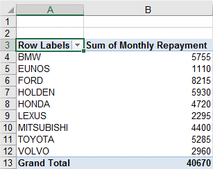
Microsoft Excel’s Pivot tables are used to summarise and group data by sum, average or Count. When creating a Pivot Table your data must be laid out correctly otherwise you will get an error message pop up.

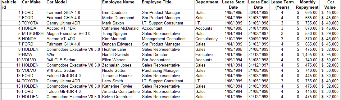
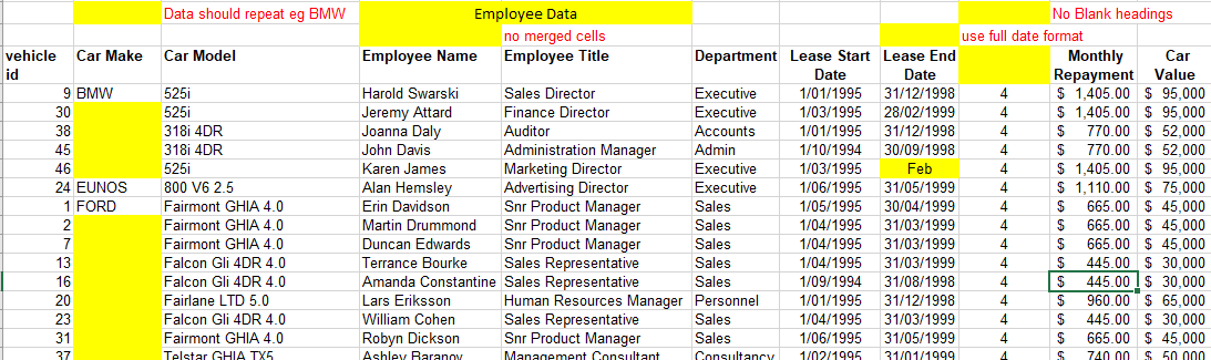
The correct format for your Microsoft Excel Pivot Table data is that the top header row must contain the field names and the consecutive rows below must contain the records of data. Do not have blank rows or blank columns. Don’t group data or add total rows.

This is a definite NO NO in Microsoft Excel Pivot Tables. No Merged data headings either.

Whenever you can use “Format as Table” for your data format this will have great benefits and save time. To start a Microsoft Excel Pivot Table ensure your cursor is inside the data set, so long as your data has no blank rows or blank columns you should have no trouble going to the Insert Tab and Selecting, Insert Pivot Table as it will automatically pick up the block of data.

If you have decided to use Format as Table, the table name will display here.

Mac’s also have the Format as Table feature.

Fields To Display In Pivot Tables

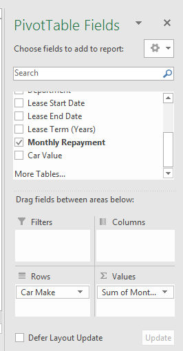
From the field list that now displays on the right hand-side choose a broad category to group by, like State or Department, because this field is a text field when you tick it – it will display in the row items.

Next choose a numerical piece of data to group by, like “Total Amount” or “Inc GST Amount”. Sometimes the Total Amount field may position itself in the row field instead of the Values field or calculate the count instead of Sum. In this case simply drag and drop the field to the Values Item.

At times the Pivot Table registers a field as a count instead of sum, Right Mouse Click on a figure in the Pivot Table and select Number Format.

For data will large number of column headings try creating a VLOOKUP to shorten the number of columns you see in your Microsoft Excel Pivot Table Field List.

Ensure your cursor is in the data set before you go to the Insert tab and Select Pivot Table.

Correct Data Layout

Incorrect Data Layout

Remove Classic Pivot Table View

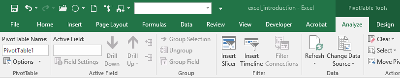
Do you still like your classic view in Pivot Tables in Microsoft Excel, or do you prefer the modern view but can’t get out of the classic view? In version 2013, 2016 you will find in the Microsoft Excel Ribbon that it is now called Analyze instead of Options. Look for the options command usually found to the left of the Ribbon.

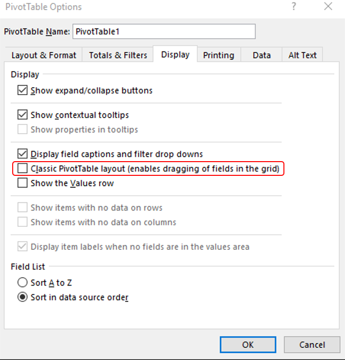
Remember in Microsoft Excel versions 2007 and 2010 you will find it under the tab call Options and then again you are looking for a command button called Options. From the Display tab in the dialog box, you will need to Un-tick or Tick as you like “Classic Pivot Table layout” which enables you to drag and drop fields into the Column and Row items area.

Creating functions to incorporate dynamic data is something you would have done in the past but now in Microsoft Excel Pivot Tables, there is a feature in Microsoft Excel versions 2010, 2013 and 2016 which now has “Format as Table” allowing your data to increase as you add more records – “rows of data” and add new fields – “columns of data”.

This means you don’t have to go to the data source consistently to add those extra few rows of data or new columns of data.

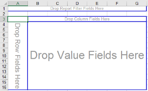
Microsoft Excel Version 2003 Classic Pivot Table Display view.

Microsoft Excel Version 2016 Ribbon

Microsoft Excel Options Dialog Box

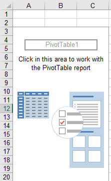
Microsoft Excel Version 2007 to 2016 Pivot Table Standard Layout Display

Creating A Quick Pivot Chart

Ensure your cursor is in side a cell of the Pivot Table. Your Pivot Chart gets its information from a Pivot Table and the Pivot Table gets its information from the raw data.

In a hurry and needing to produce an Excel Chart. Select your data then Press F11. Your chart will be created in a separate sheet. Press Alt F1 to create the chart in the same sheet.

Mac user no Wala your F11 key performs a different function. Remember when you make changes to the Chart they will make changes back to the Pivot Table. When you make changes like play with filters in the Pivot Table they will change the chart.

Beyond Pivot Tables

There are other tools more powerful than Pivot table explore Power Pivots which now come with MS Office 2013 – Excel. Power Pivots allow you to create Pivot Tables from multiple tables and create a relationship all while not importing into Microsoft Excel cells.

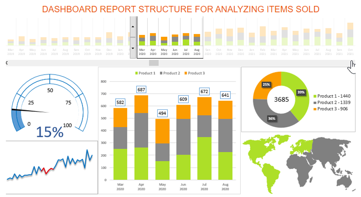
Meaning you are not limited to over 16,000 fields/ headings or over 1 million records. There are also Power Queries and Power Bi which almost work like a database and then can generate Dashboards. Dashboards are visualisations meaning a collection of graphs to display large amounts of data more clearly and simply.

Conclusions

Use Pivot tables if you have a large amount of raw data to manipulate and you want to get statistical information. Groups like information together.

Viewing by years, categories, gender etc. Your raw data structure is important to the success of your Microsoft Excel Pivot table.

Mathematical and grouping needs are satisfied with Pivot Tables.